Motivation

In this paper, we derive a minimalist diffusion model. The diffusion model that we obtain is pretty much equivalent to existing ones but the whole point is the derivation that, we believe, is simpler than the existing ones.

Indeed, when we started learning about diffusion models, we found it pretty hard to enter the topic. There were many new concepts to learn: Langevin dynamics, score matching, SDEs, etc. Even basic tutorials that are supposed to provide simple overviews of the concepts turn out to be pretty complicated and math-heavy.

So, we decided to derive our model from scratch, using only basic (bachelor-level) concepts. This is what our paper is about. It is the one we wish we were given when we started learning about this topic.

Overview

Technically, the whole point of the method is to compute a deterministic mapping between the samples of two arbitrary distributions: $x_0 \sim p_0$ and $x_1 \sim p_1$. In the below figure, $p_0$ is illustrated as a red triangle and $p_1$ illustrated as a green square. The deterministic mapping connects each $x_0$ to a unique $x_1$. Hence, generating random samples $x_1 \sim p_1$ can be achieved by generating random samples $x_0 \sim p_0$ and evaluating the mapping.

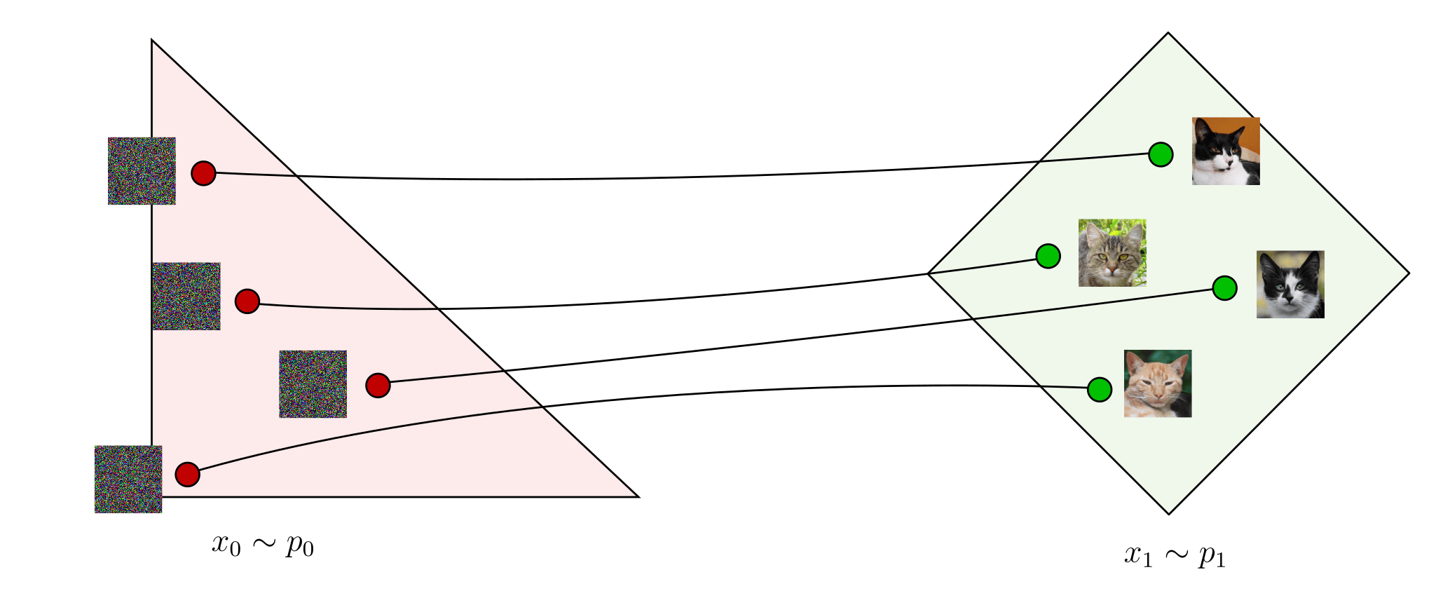
These examples are 2D but it works the same in high-dimensional image spaces. For instance, $p_0$ could be a Gaussian noise distribution and $p_1$ a distribution of cat images. If we can compute a deterministic mapping between the Gaussian noise images and the cat images, then we can sample random cat images by generating random Gaussian noises and evaluating the mapping. So, how do we define and compute such a mapping?

The theory: blending and deblending iteratively creates a deterministic mapping

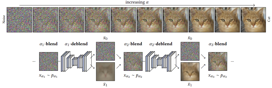
Our deterministic mapping is based on a sampling interpretation of α-blending: what happens statistically when we linearly blend and deblend points (or images)? We consider two basic operations: α-blending and α-deblending shown in the figures below:

$\alpha$-blending

$\alpha$-deblending

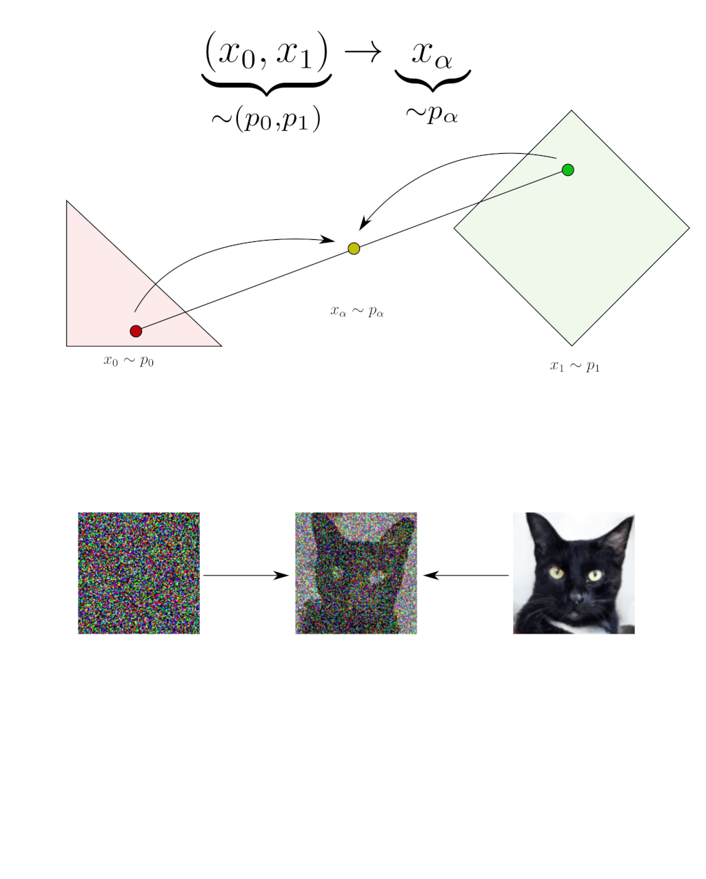
What we call α-blending is linearly interpolating random samples in the following way:

For instance, blending a random Gaussian noise $x_0 \sim p_0$ and a random cat image $x_1 \sim p_1$ with parameter $\alpha$ produces a noisy cat image $x_{\alpha} \sim p_\alpha$. We note $p_\alpha$ the distribution of the noisy cat images that can be randomly sampled in this way. Statistically, blending is a transformation that goes from $\left(p_0, p_1\right)$ to $p_\alpha$.

Deblending is the inverse statistical operation. For a given blended sample $x_{\alpha}$, deblending consists of recovering a $x_0$ and a $x_1$ that could have been α-blended into this $x_{\alpha}$. Note that there are usually multiple possibilities. In this example, different Gaussian noises $x_0$ and cats $x_1$ could have been α-blended into the same noisy cat $x_{\alpha}$. Deblending means choosing one of these couples $(x_0, x_1)$ at random. Deblending is thus the inverse operation of blending in the statistical sense, it is not the samples that are inversed but their statistics: deblending is a transformation that goes back from $p_\alpha$ to $\left(p_0, p_1\right)$.

An important point is that this deblending operation is not something one can actually do. How to recover a $x_0$ and a $x_1$ that could have been α-blended into a given $x_\alpha$ is a difficult problem in general. Fortunately, it is just a theoretical consideration useful for the derivation and we will never need to do it in practice. So, for now, just assume that we can do it.

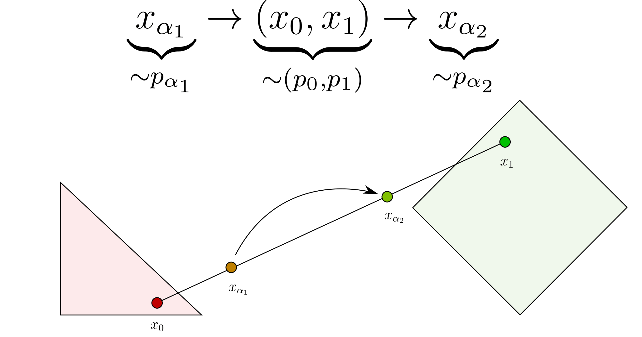
Now that we have blending and deblending, we have the two main ingredients to construct our deterministic mapping. The idea is that chaining them allows for navigating between the $p_\alpha$ distributions. For instance, in the above example, we start with a sample $x_{\alpha_1} \sim p_{\alpha_1}$. By deblending it, we obtain a couple $(x_0, x_1)$, such that we are back in the orginal distributions $\left(p_0, p_1\right)$, and by reblending with a different parameter $\alpha_2$ we obtain a sample $x_{\alpha_2} \sim p_{\alpha_2}$. As a result, by chaining deblending and blending we have statistically navigated from $p_{\alpha_1}$ to $p_{\alpha_2}$. Note that there are no constraints on $\alpha_1$ and $\alpha_2$, they can be arbitrarily close or distant.

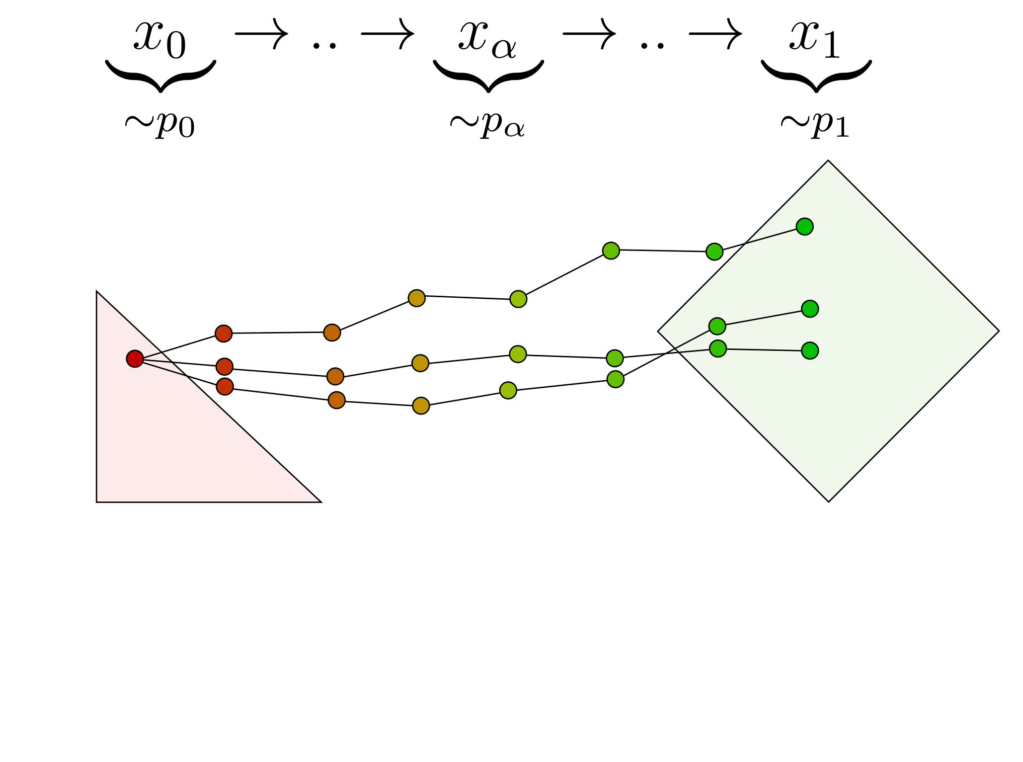
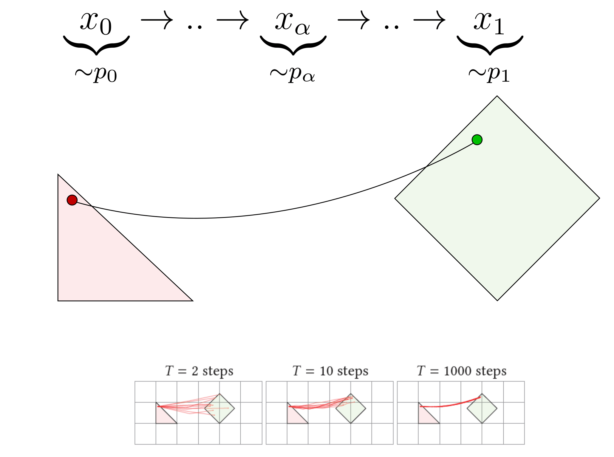
Our deterministic mapping emerges when we do that multiple times iteratively with increasing $\alpha$ values. For instance, we can compute 6 steps with $\alpha=0.0, 0.2, 0.4, 0.6, 0.8, 1.0$. This creates a discrete random path that connects a $x_0 \sim p_0$ to a random $x_1 \sim p_1$. However, the path is stochastic, since each step is random. So, each time we run the algorithm again, the path is different and $x_0$ is connected to a different $x_1$.

The main discovery of the paper is that, the more steps we use, the more the stochasticity of the path disappears until it finally converges to a deterministic path. Intuitively, this is because, each step is random and as we increase the number of steps, their randomness simply averages out. This is a simple consequence of the Central Limit Theorem: averaging many random things removes the randomness and coverges towards their expected value. The limit of the iterative α-(de)blending algorithm is thus a deterministic mapping that deterministically connects each $x_0 \sim p_0$ to a unique $x_1 \sim p_1$.

The practice: learning and evaluating the mapping with a neural network

Now, remember that computing this deterministic path is not practical yet because we need to use the (non-practical) deblending operation for each step. Fortunately, in the infinitesimal limit, the non-practical deblending operation disappears!

Indeed, let’s have a look at what happens when we compute an infinitesimal step that maps $x_{\alpha} \sim p_\alpha$ to $x_{\alpha+\Delta\alpha} \sim p_{\alpha+\Delta\alpha}$:

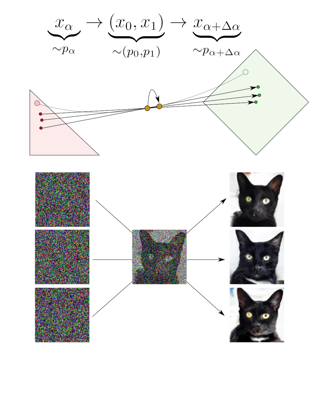
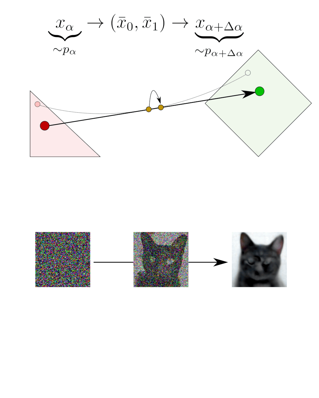
The deblending operation at $x_\alpha$ requires considering all the couples $(x_0, x_1)$ that could have been blended into this $x_\alpha$, choosing one of these couples $(x_0, x_1)$ and performing the infinitesimal step $\Delta\alpha$ along the segment $x_1-x_0$.

Fortunately, in the infinitesimal limit, these small steps average out. As a result, moving along one of the random segments $x_1-x_0$ becomes equivalent to moving along the average of these segments. In other words, the average segment $\bar{x}_1 -\bar{x}_0$ is the tangent of the deterministic path. If we can compute this tangent in practice, we can move along the deterministic path.

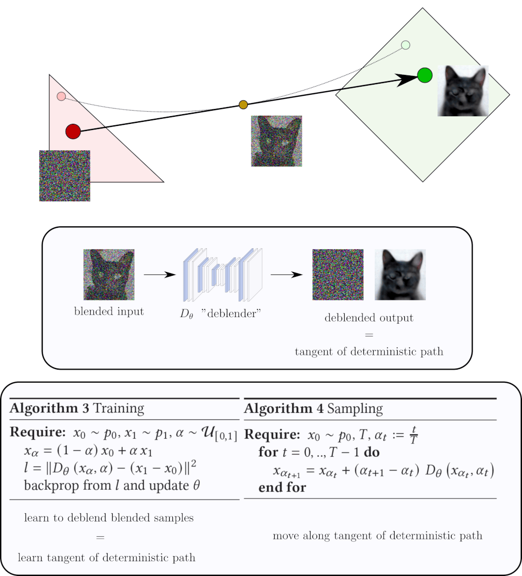
This is where the neural network comes into play. The idea is to train a neural network to deblend blended samples. The key point is that, as we have seen, for a given blended sample $x_\alpha$ there are always multiple possible outputs $(x_0, x_1)$ that could have been blended into $x_\alpha$. What does the neural network learn when one input can produce different outputs? That depends on the training loss. If we train the neural network with a $l_2$ norm, it learns the average of the multiple outputs (the tangent of the deterministic path), which is precisely what we want.

In summary, we train a neural network to deblend blended samples, which makes it learn the tangent of the deterministic path. Once the training is over, we generate images by starting with an $x_0$ and we follow the deterministic path iteratively by moving along the tangent predicted by the neural network. That’s it! We obtain a deterministic diffusion model that is, in essence, equivalent to the state-of-the-art deterministic diffusion models.

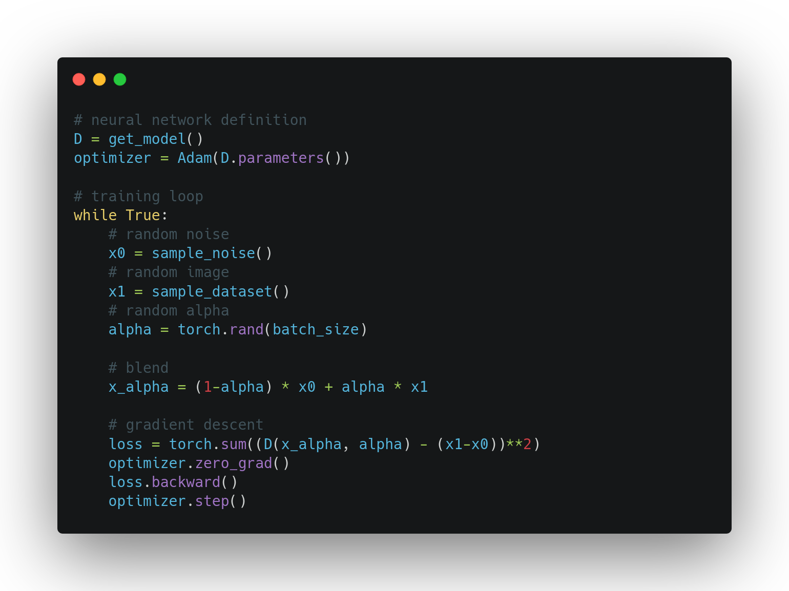
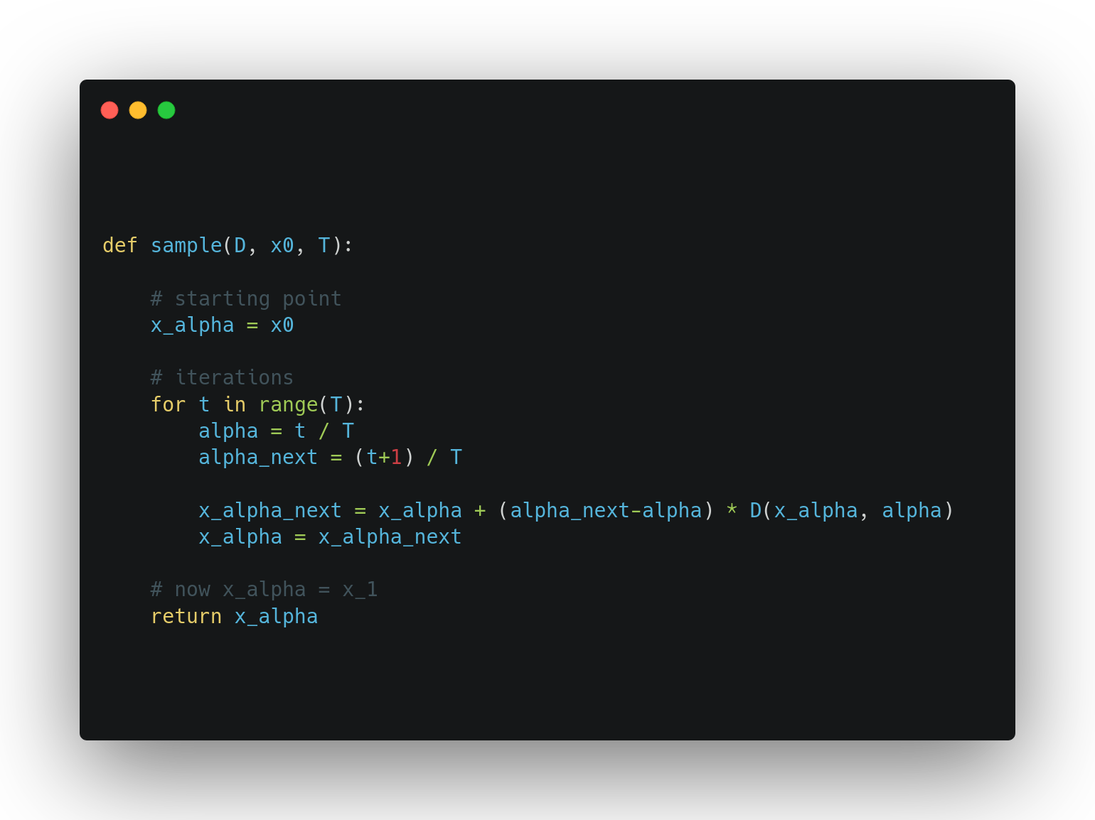
Herebelow is a pseudocode implementation of the training and sampling algorithms.

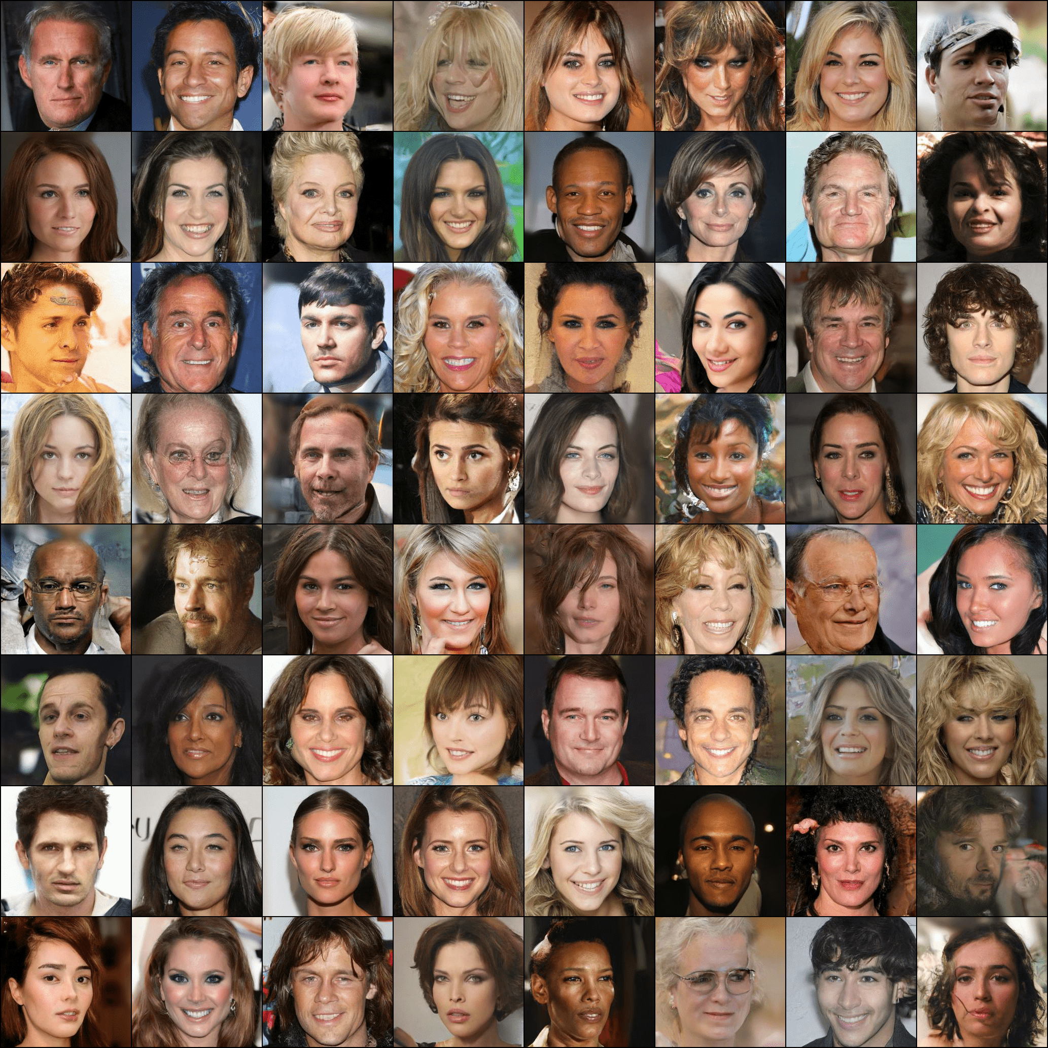
Application: Image Generation

We apply our formulation to image generation of image dataset such as the CelebA dataset. Herebelow we display an uncurated grid of images outputed using the sampling algoritm above:

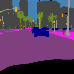
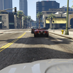
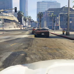
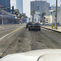
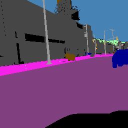
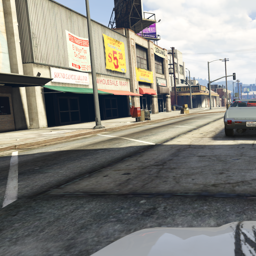
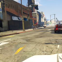
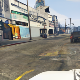
We also show in our paper examples of conditional image generation. Below are two examples of conditional models:

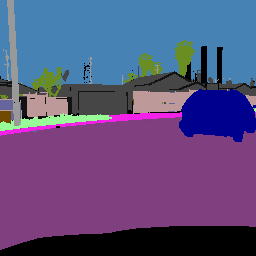
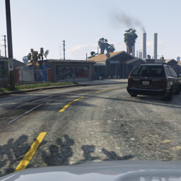
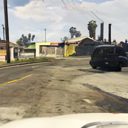
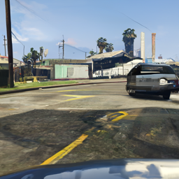
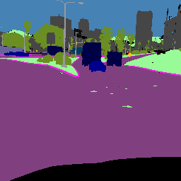
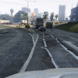
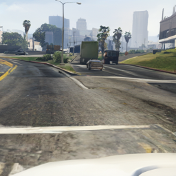
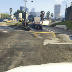
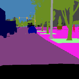
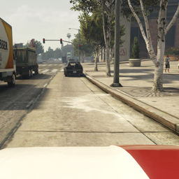
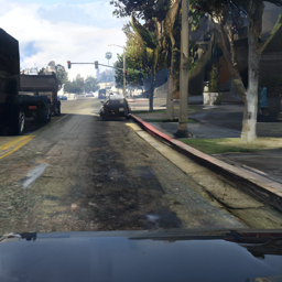
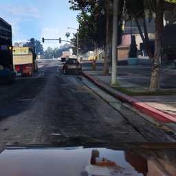
GTA V

Input	Reference	Generation 1	Generation 2

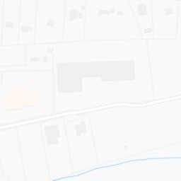
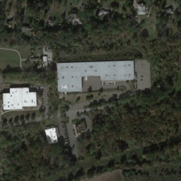
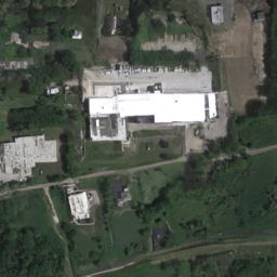
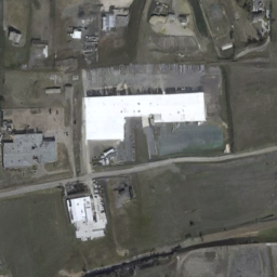
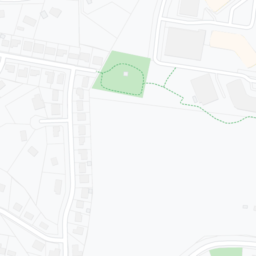
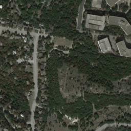
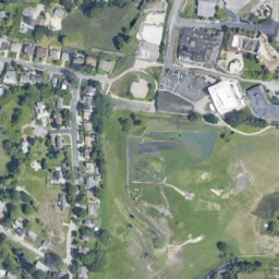
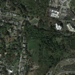
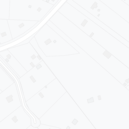
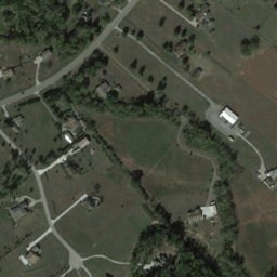
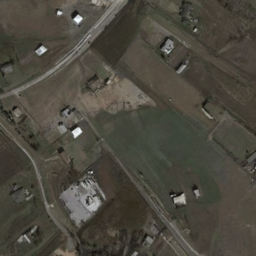
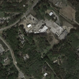
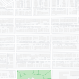
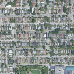
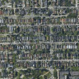
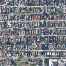
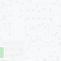
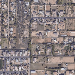
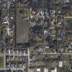
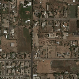
Map2Sat

Input	Reference	Generation 1	Generation 2